Datasets
We used previously developed RB198 dataset of 198 RNA-binding protein PDB chains (Walia et al., 2012). Resolution of all chains is better than 3.5 Å and sequence identity between all chains is less than 30%. Cut-off distance of 5.0 Å was used to determine the RNA-interacting and non-interacting residues. A residue was considered to be interacting if the closest distance between residue and the partner RNA was within the cut-off (5 Å). All remaining residues were considered as non-interacting residues. All remaining residues were considered as non-interacting residues. RB198 dataset contains 7950 RNA-interacting and 45710 non-RNA-interacting residues from the total of 53660 residues.
In order to evaluate performance of our prediction models on an independent dataset, we used a previously developed RB44 dataset (Puton, Kozlowski, Tuszynska, Rother, & Bujnicki, 2012). RB44 contains 40% non-redundant chains of 44 RNA-binding proteins. At the 5.0 Å cut-off distance, it contains 1956 RNA-interacting and 4521 non-interacting residues. All RIRs were considered as positive and all non-RIRs were considered as negative instances.
Overlapping window patterns
We generated overlapping (sliding) window patterns of different sizes from protein chains. The sliding window patterns based strategy has been used in many studies for annotating proteins at the residue level, Therefore we used the same 25-residue long window size for prediction of RNA interacting mono-residues (RIMRs), where if the central (13th) residue of a pattern is interacting then the whole pattern was assigned as RIMRs (positive) pattern, otherwise it was assigned as the non-RIMRs (negative) pattern. Likewise, we used 26, 27, 28 and 29-residue long window sizes, where if the central two (13th and 14th), three (13th, 14th and 15th), four (13th, 14th, 15th and 16th) and five (13th, 14th, 15th, 16th and 17th) residues were RNA-interacting then patterns were assigned as RNA interacting di-residues (RIDRs), tri-residues (RITRs), tetra-residues (RITTRs) and penta-residues (RIPRs) respectively, otherwise assigned as non-RIDRs, non-RITRs, non-RITTRs and non-RIPRs respectively. In order to generate patterns for terminal residues, we added dummy X residue at both ends of (N-1)/2 lengths for 25,27 and 29 length window size and N/2 for the 26 and 28 window size, where N is a size of the pattern. We used only those negative patterns from RB198 dataset, where interacting residues were completely absent in the whole pattern.
Patterns generated from RNA binding proteins (as described above) cannot be used directly for developing models-- as machine learning techniques based models need fixed length numerical patterns rather than peptides. Therefore we applied different approaches for the development of different SVM-based prediction models.
Binary Profile of Patterns (BPP)
In the residue level prediction, BPP approach is commonly used approach. In this, positive and negative patterns were converted into the binary profile of patterns. Where all amino acids represented by a unique vector of 21 dimensions (e.g. Ala by 1,0,0,0,0,0,0,0,0,0,0,0,0,0,0,0,0,0,0,0,0; Cys by 0,1,0,0,0,0,0,0,0,0,0,0,0,0,0,0,0,0,0,0,0), which contained 20 standard amino acids and one dummy amino acid “X”.
Composition Profile of Patterns (CPP)
The different length of overlapping (sliding) patterns were created from protein sequences of datasets. The amino acid composition of each pattern was calculated. These composition profile of patterns have been used for the SVM-based machine learning and model development.
PSSM Profile of Patterns (PPP)
The PSSM based approach has been applied in various residue level prediction methods. We used PSI-BLAST (position-specific iterative BLAST) search against the Swiss-Prot database (at default parameter). The PSSM profiles were generated from multiple-alignment of high-scoring hits after three-iterative search. These PSSM profiles contain the position-specific scores of occurrence probability of all amino acids at each position in the alignments. We used complete query protein to search against Swiss-Prot, generated PSSM profile and thereafter extracted patterns wise PSSM score. Finally, we used PSSM score after Min-Max normalization.
SVM
Support Vector Machine (SVM) is a highly successful machine learning technique for biological predictions. We used SVM_light package for the development of RNAint. We optimized different kernels and parameters. The svm_learn software used for training of model. After training, learned model used for prediction of unknown/test examples using svm_classify.
Evaluation Methods
In this study, performance of SVM modules were evaluated using a 5-fold cross-validation technique. In the 5-fold cross-validation, the relevant dataset was randomly devided into five equally sized sets. The training and testing was carried out five times, each time using one distinct set for testing and the remaining four sets for training. The performance of the methods was computed using the following formulas :-
Sensitivity = (TP / (TP+FN))*100
Specificity = (TN / (TN+FP))*100
Accuracy = (TP+TN / (TP+FP+TN+FN))*100
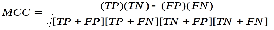
Where TP and TN are correctly predicted RIRs and non-RIRs respectively. FP and FN are wrongly predicted RIRs and non-RIRs respectively.
Probability Score
The RNAint gives a probability score for each residue of sequence. The probability score is a measure of correct prediction. Where SVM score of more than 1.5 and less than -1.5 fixed with 1.5 and -1.5 respectively. The probability score varies from 0-9 for each residue of protein sequence. The probability scores ranges between 0-4 and 5-9 predicted as non-RIRs and RIRs respectively (at 0.0 threshold).